Making a Pixel Classifier
Go to the bottom of the page for a list of useful links to packages / algorithms used in this module of PalmettoBUG.
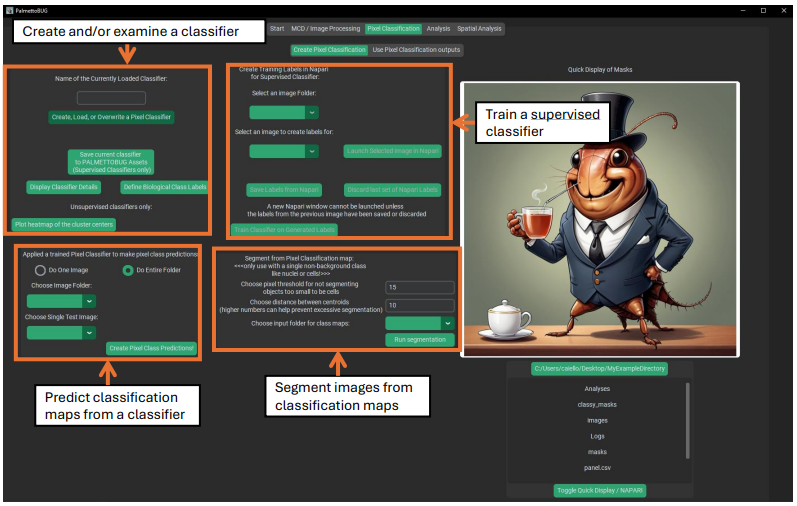
Pixel classifiers are made in the first sub-tab of the Pixel Classification tab:
What is a Pixel Classifier?
Pixel classifiers are algorithms that can group the pixels of your images into classes – these classes can be connected to biologically relevant groupings and be used to variety of things, including transforming images, transforming masks derived from those images, and labeling cells derived from the masks + images.
These classifiers come in two main flavors – supervised and unsupervised classifiers – which differ in how they are trained and the kind of outputs they create.
Creating Supervised Classifiers
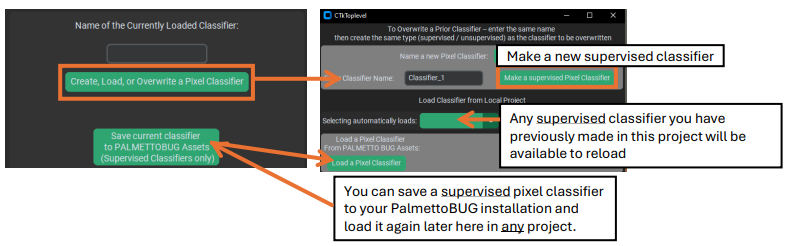
To make any classifier, click on the “create, load, or overwrite” button in the upper left corner. This will launch a window where you can choose to either create a pixel classifier (supervised or unsupervised), or load a classifier. Classifiers can be loaded from the project– any classifier made in an imaging project will be automatically saved & available for reload inside that project – or from PalmettoBUG itself. Supervised classifiers can be saved to PalmettoBUG, making the classifier then available to any project run in that installation of PalmettoBUG. Only supervised classifiers can be reloaded in such a way that they can predict new outputs – unsupervised classifiers can be loaded, but only for the purpose of examining their setup details and predictions.
Once you have chosen to create a new supervised classifier, a new window
will open where you can select the settings for it. 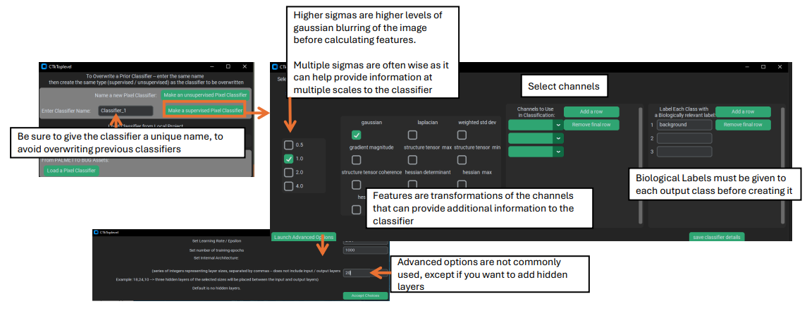
Key settings for a supervised classifier include:
1). Sigma(s) – these values control the level(s) of Gaussian blurring that is applied to the channels while creating features layers. Multiple sigmas can be selected, and this is often recommended as it means that the classifier will receive information from multiple scales of the data, since higher sigmas (greater blurring) will contain more global / non-local information in each pixel, while features generated from lower sigmas will contain less blurred / more local information.
2). Feature(s) – these are transformation to the image channels which can derive more information in addition to the plain intensity values. ‘Gaussian’ is included by default as it is analogous to the raw intensity of the image, just smoothed and blurred by the chosen sigmas. The other features do more radical transformations of the data that do not correspond to raw intensity. For example, Hessians (especially the Hessian minimum) and the Laplacian use kernels that calculate derivatives of the image, and can help identify edges or areas of sharp transition in a channels’ intensity – but not the intensities themselves. The implementation of these features was directly translated from QuPath into python, and you can see QuPath’s documentation for more information about the available features and why you might use them: Pixel classification — QuPath 0.5.1 documentation. One piece of advice from the link above copied here: “…it can be much more effective to use a smaller number of well-chosen features rather than throwing them all in to see what comes out the other end.”
3). Channel(s). These are straightforward – they are the channels that will be blurred and transformed to generate the sigma / feature layers fed into the classifier. Like the features, it is often best to stick to a small number of high information channels than to include channels with poor signal / limited relevance to the classifier’s desired output. Additionally, using fewer channels saves a lot of computation: the number of layers calculated & passed into the neural network during training and prediction is:
# of data layers = (# of sigmas) * (# of features) * (# of channels)
This is because for each channel selected, every selected feature will be created at every selected sigma, then all those layer of the image will be joined together into a large array and fed, pixel by pixel, into the neural network for training / prediction.
4). Classes. These are the categories that you want to predict in the image. For supervised pixel classifiers, the first class is ALWAYS background and gets treated differently than the other classes. Typically, it is best to make classifier’s that predict one class at a time if the classes are not mutually exclusive – for example, if you make a classifier for two different ECM proteins (let’s say collagen and vimentin), since the two could be in the same location in the image at once it is better to do two different classifiers (unless you add a dedicated double positive class). However, if you want to find multiple classes are mutually exclusive (such as different cell types), then a single classifier may be preferrable.
Note
Images are arrays of numbers, so when the classifier makes pixel predictions and saves them as an image, it will be as numbers, and not the class labels. Use the classifier details button, or look at the biological_labels.csv in the pixel classifier’s folder to see how the numbers in the pixel classification maps correspond to the biological labels that you assigned.
Creating Training Labels in Napari
Supervised classifiers are distinct from unsupervised classifiers because they require more user input than unsupervised classifiers. Specifically, supervised classifiers require the user to create training labels in Napari. To do this, first launch an image in Napari, then use Napari tools to create a label layer, finally close Napari and click the save labels button in PalmettoBUG. In is other a good idea to open the details window with the “Display Classifier Details” button before launching in Napari, as it will contain the information needed to match channel / label numbers to the desired channels / labels.
Warning
While Napari is open in this step (this does not apply when Napari is opened by other steps / methods in PalmettoBUG), the PalmettoBUG windows will be non-responsive, and if you try to move a PalmettoBUG window the entire program may crash! This error is because of how Python handles threads. So open any windows you may need (like the classifier details) BEFORE launching training labels in Napari, and do not try to move these PalmettoBUG windows while Napari is open (minimizing/maximizing it should be OK, though)!
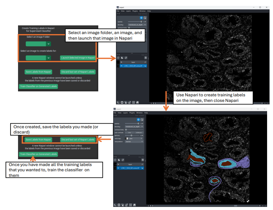
When you launch an image for training creation, you should see two image-stacks in the middle-left side of the window, one named “layer” on top, and the other named after the image that you launched on the bottom. You will want to use the slider at the bottom of the Napari screen to select the desired channel, and if you need to change the thresholds for that image click on the bottom image-stack to gain access to those controls.
Once you are on your desired channel, be sure that the top image-stack (“layer”) is selected, to gain access to the labeling tools in the upper-left. You will want to set the label to the number you are going to make training labels for (remember background = 1, etc.), and then select the paintbrush icon above the label number to begin labeling the image. Change the brush size and use the erase icon for fine control of the labeling. Repeat for every label in the classifier – while not every image has to have labels for each class, there MUST be some labels for each class available in the training dataset, and usually every class is present in every image.
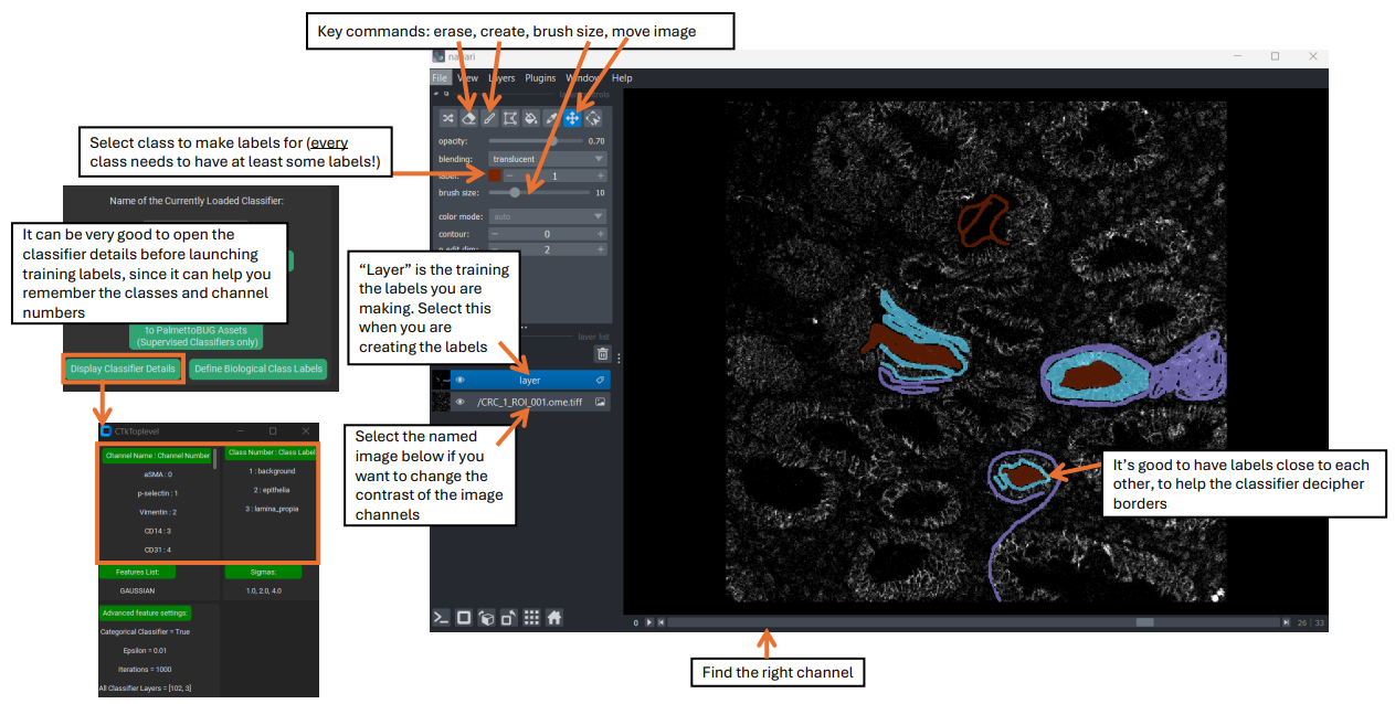
Then, repeat the Napari launch / labeling process for as many images as you want. The more images you do, especially if there are diverse fields of view in the data, then hopefully the more competent the classifier will be at handling all the diverse images of your project. In general, it is good to make labels in multiple locations and contexts across the images, and to have different classes’ labels next to each other at least some of the time, since labeling the border regions between classes can help the classifier better distinguish between the classes.
Finally, once you are satisfied with the labelings that you have created, train the classifier.
Note
The set of images that the classifier will be trained on is set by the image folder selected when launching images for training label generation – if you change that folder between creating the training labels and training the classifier, then the images used in training will be different from the images you used to make the training labels!
Prediction
Once a supervised classifier is trained, one or more images can be predicted. First select a folder – in most cases, this should be the same folder on which the classifier was trained – i.e., if you trained your classifier on the images in the denoised image folder, you should predict with those images, too.
Next, set the prediction to do the entire folder of images or just one image. If only predicting from one image is selected (which can be useful to get a quick look at how the classifier appears to be performing without needing to wait for the entire folder to be run) then use the drop-down menu for selecting an image. This drop-down is ignored if you choose to predict the entire folder.
Finally, run the prediction!
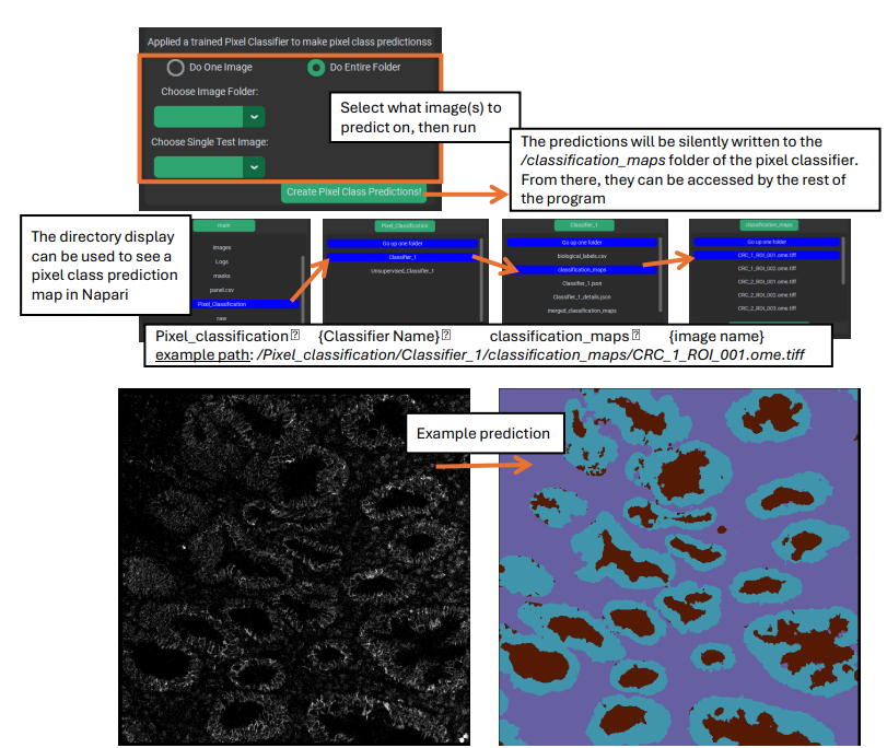
The predictions are written to the pixel classifier’s /classification_maps sub-folder, where they are accessible by the rest of the program for downstream steps. However, they are not automatically displayed after prediction.
You will want to examine your pixel class predictions to see if they are capturing the classes that you want accurately, and to do this you should launch the classification map(s) in Napari. This can be done in the directory display from inside PalmettoBUG, or you can open Napari in a separate terminal from PalmettoBUG and navigate to the relevant directories using your system native file managing app. If you use the directory display inside PalmettoBUG’s pixel classification tabs, then the source image will also be loaded into Napari beneath the classification prediction, allowing you to easily go back and forth between the pixel class predictions and the original image.
Creating Unsupervised Classifiers
Unsupervised classifiers are an interesting alternative way to classify pixels. The implementation is inspired / derived from the Pixie / ark-analysis / toffy software from the Angelo lab. See this GitHub repository for details of their package: angelolab/toffy: Scripts for interacting with and generating data from the commercial MIBIScope
The specific way these classifiers work is that a subset of all the pixels in the images are sampled, and a FlowSOM is trained on that subset, fitting to find a user-defined number of metaclusters in the data. Then, that subset-trained FlowSOM can be used to predict ALL the pixels in the images. Before being used for training / prediction, the intensity values of the pixels are normalized within each channel by dividing all by the 99.9% quantile, followed by normalizing within each pixel (designed to follow the normalization steps used in Pixie / toffy).
Unsupervised classifiers operate with a few key differences from supervised classifiers:
1). Training inputs. While supervised classifiers require training labels made by the user, unsupervised classifiers train directly on a sample of the pixels without needing any similar supervision. This is why the two types of classifier are named the way they are.
2). The output classes of an unsupervised classifier have no biologically-relevant label (the classes must be annotated / merged after the classifier is run). This is because, without supervision, these classifiers merely clump similar looking pixels together without any understanding of the biological label that might apply to each group – that must be supplied by the user.
3). Unsupervised classifiers tend to output more classes. While this is really under the control of the user, typically unsupervised classifiers should create much more classes than a supervised classifier – any excess / redundant groups can be annotated and merged together later. Overall, unsupervised classifiers use the same FlowSOM merging process that is typically utilized to find cell types in the Analysis tab of the program.
4). Some of the hyper-parameters for training are different between the types of classifiers. More detail on these in the next section.
5). Unsupervised classifiers must be used for prediction when they are created, i.e. they cannot be saved and re-used. They can be saved and reloaded for the purposes of viewing their original training / setup details, but they cannot be reloaded & run again. If you need to duplicate a prior unsupervised classifier, you must use the first classifier’s details to create an identical copy, retrain it, and then you can proceed with using / predicting from the duplicate.
6). The output of unsupervised classifiers tends to be more prone to find isolated / discontinuous regions of pixel classes. This is likely in part because the higher number of classes predicted and in part because there is not a smooth / continuous training set of pixels as is typical with the human-provided inputs for supervised classifiers. This abundance of small, isolated, or discontinuous pixel class regions makes their baseline output harder to use for most applications except classifying cells using a secondary FlowSOM. These problematic regions can also be partly controlled by using the “smoothing” option during class prediction.
Creation
Creating an Unsupervised classifier starts similarly to creating a supervised classifier – using the same button in the upper left to launch the ‘create a classifier’ window. But once in this window, use the button for creating an unsupervised classifier, which will launch a new window. Note that whatever name you choose for the classifier will have “Unsupervised_” appended to it. As in, if the name you select is “Classifier_1” (the default), the actual name will be “Unsupervised_Classifier_1”. This helps keep the two types of classifier distinct and clearly labeled, and assists PalmettoBUG in identifying which category a re-loaded classifier is.
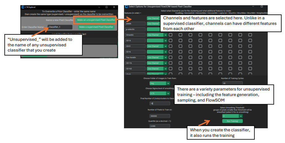
Once you are in the unsupervised classifier creation window, you will be presented with a large number of options:
1). Channels & features. Much like supervised classifiers, you must select which channels will be used for training / prediction, as well as what features to use for each channel. Unlike supervised classifiers, it is possible to have different features for different channels. Additionally, the ‘Gaussian’ feature is ALWAYS used for every selected channel (which is why it is not visible in the list of features).
2). The image folder for training and number of pixels to sub-sample. Unlike supervised classifiers, there does not need to be any training labels, but instead a subset of the pixels in the images themselves are used.
Note
Excessively large values for the pixel sub-sampling, combined with too many selected features / channels, can cause excessive use of computer memory, and if the number is too large, you may crash your computer!
3). Sigma blurring & Quantile normalization. These affect the features passed into the classifier. Specifically, the sigma value is similar to the sigmas in a supervised classifier – it controls how blurred the channel features are – except for unsupervised classifiers only 1 sigma is allowed. The %quantile normalization number determines how the data are normalized within each channel (default all channels are divided by their 0.999 / 99.9% quantile values).
4). FlowSOM parameters (metacluster number, XY dimensions, training iterations). These control how the FlowSOM algorithm is created and trained. The most critical of these is the metacluster number, as this determines the number of classes in the final predictions. The XY dimensions value controls the size of the FlowSOM grid (XY dims squared must be greater than the number of metaclusters, but fewer than the number of pixels trained on), and greater training iterations can improve the stability of the FlowSOM, although it takes more time to train.
5). Random seed. This is needed for reproducibility of both the random sampling of pixels in the images as well as the random initialization of the FlowSOM grid.
6). Smoothing. If > 0, then a custom “smoothing” procedure is performed immediately after prediction, where any pixel class region smaller than the smoothing number (i.e. fewer than that number of pixels) will have its values replaced by the statistical mode of the values of the surrounding pixels. This mode for a given pixel is calculated by looking first at the immediately adjacent pixels to calculate the mode (if all of those pixels had been part of an isolated region and also dropped, then the mode is calculated for an expanded area).
‘Run Training’ from this window completes the creation of the classifier. This step can take a while to complete, as it will be performing channel normalizations, pixel subsampling, and FlowSOM training.
Prediction
Prediction is performed in the same way, and using the same GUI buttons, as for supervised classifiers. You select an image folder (this should essentially always be the same folder that you trained the classifier on), choose whether to predict the entire folder of images or just one image, and then if applicable select the single image to classify.
Note
Unlike supervised pixel classifiers, unsupervised classifiers cannot make class predictions after being reloaded, you must make the predictions the first time you create them – they can be reloaded in order to do things like examine their training parameters, but not for prediction.
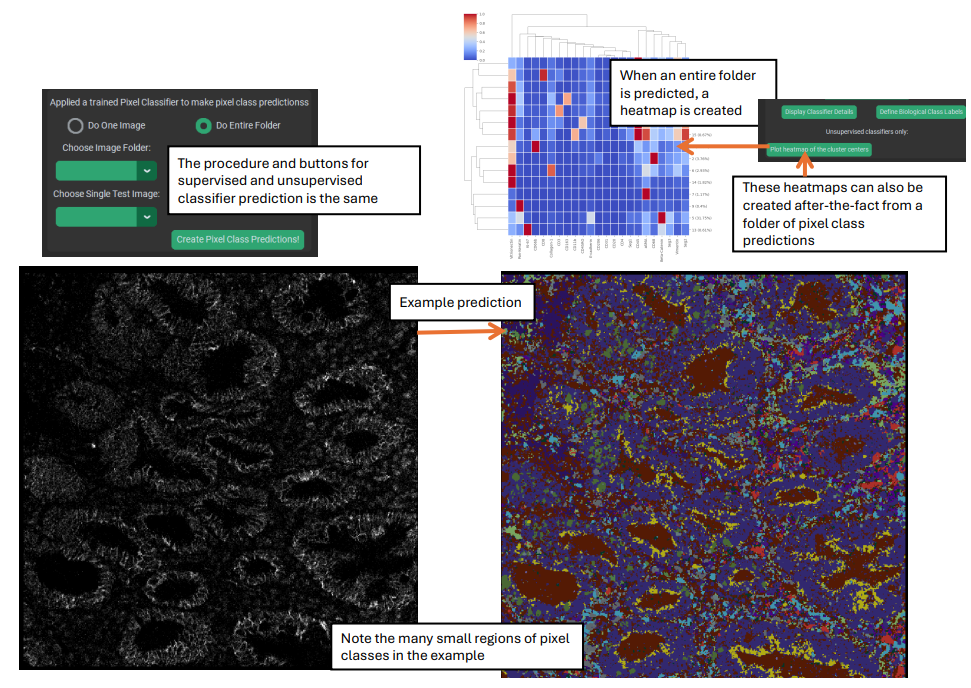
When an unsupervised classifier makes a prediction for an entire image folder, a heatmap is automatically generated at the end (this heatmap can also be made using the “Make heatmap from previously created predictions” button in the upper left frame). This heatmap gives an idea of the expression of the selected channels in each predicted class of the classifier, and is a key plot for helping to annotate and merge the predicted classes.
Annotation and merging
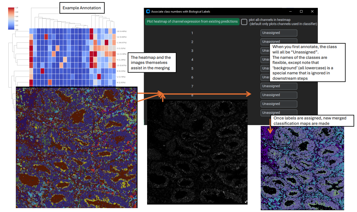
When you accept the new labels, a new folder (merged_classification_maps) is created in the pixel classifier directory, where the merged class predictions are written. Specifically, any class in the original classification maps that was labeled as ”background” is set to 0 in the merged maps, and every group of classes that share the same label are merged together to a single unique identifying number. These new numbers are kept track of by the biological_label.csv file.
Segmentation from a classifier
Why is this section in the document about making a classifier, and not in the documentation about using a pixel classifier? Because I say so, that’s why!
In addition to my dictatorial whim, the segmentation controls were originally placed in the classifier creation tab because limited space for the widgets in the pixel usage tab – and that still hasn’t been changed yet.
Segmenting with a classifier is not a procedure you will typically want to do, except in very particular circumstances. Usually, the generalist models Cellpose / Deepcell will be sufficient and superior for segmentation. However, if you want to segment objects that meet at least two of the following three criteria 1). well separated, 2). generally circular, 3). generally of a uniform size / distance apart, then segmentation using a pixel classifier is possible.
To do this, you will want to make a single-class supervised classifier that identifies the objects you want to segment. Once you have made predictions, you can go to the center-lower frame of widgets and select the classifier output you want to use, as well as a couple of parameters that help control segmentation mask size and location.
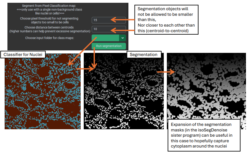
This style of segmentation is quite reasonable for things like nuclear segmentation (as usually nuclei are generally circular, well separated, etc.), and nuclear segmentation can often be followed up by expansion of the masks to approximately capture the cytoplasm around the nuclei.
Links
These are links to some packages / software / manuscripts that can be helpful to understand this page of documentation, as either code or techniques / ideas from these are used in PalmettoBUG’s pixel classifiers.